How to Create a Pie Chart in Excel in 60 Seconds or Less

Initially of 2021, I used to be tasked with an project: Create a pie chart showcasing which forms of content material carried out greatest on the Advertising and marketing Weblog in 2020.

The query was an undeniably necessary one, as it could affect what forms of content material we wrote in 2021, together with figuring out new alternatives for development.

However as soon as I might compiled all related information, I used to be caught — How may I simply create a pie chart to showcase my outcomes?

Fortuitously, I’ve since figured it out. Right here, let’s dive into how one can create your individual excel pie chart for spectacular advertising and marketing stories and displays. Plus, the right way to rotate a pie chart in excel, explode a pie chart, and even the right way to create a three-dimensional model.

Let’s dive in.

Learn how to Make a Pie Chart in Excel

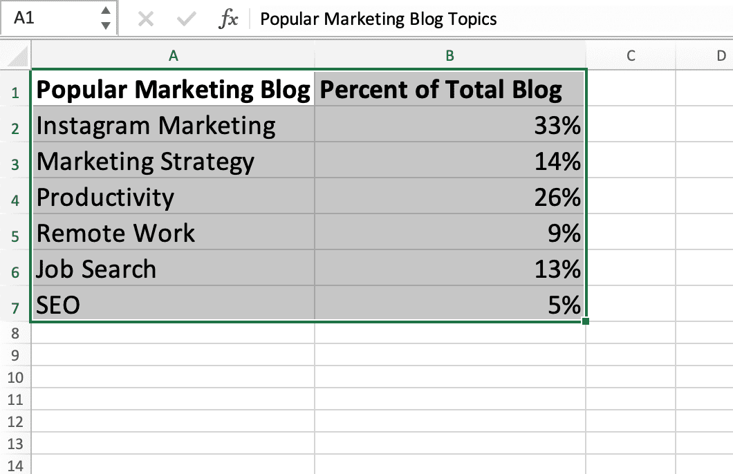
1. Create your columns and/or rows of information. Be happy to label every column of information — excel will use these labels as titles in your pie chart. Then, spotlight the information you need to show in pie chart type.

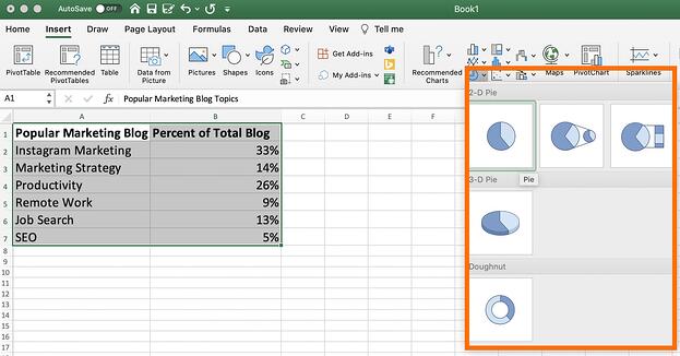
2. Now, click on “Insert” after which click on on the “Pie” emblem on the prime of excel.

3. You will see a number of pie choices right here, together with 2-dimensional and three-dimensional. For our functions, let’s click on on the primary picture of a 2-dimensional pie chart.

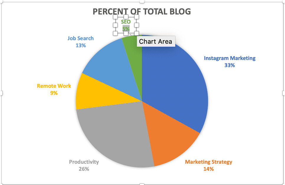
4. And there you’ve it! A pie chart will seem with the information and labels you’ve got highlighted.

In the event you’re not proud of the pie chart colours or design, nonetheless, you even have loads of enhancing choices.

Let’s dive into these, subsequent.

Learn how to Edit a Pie Chart in Excel

Background Coloration

1. You possibly can change the background shade by clicking on the paint bucket icon beneath the “Format Chart Space” sidebar.

Then, select the fill kind (whether or not you need a stable shade as your pie chart background, or whether or not you need the fill to be gradient or patterned), and the background shade.

Pie Chart Textual content

2. Subsequent, click on on the textual content inside the pie chart itself if you wish to rewrite something, broaden the textual content, or transfer the textual content to a brand new space of your pie chart.

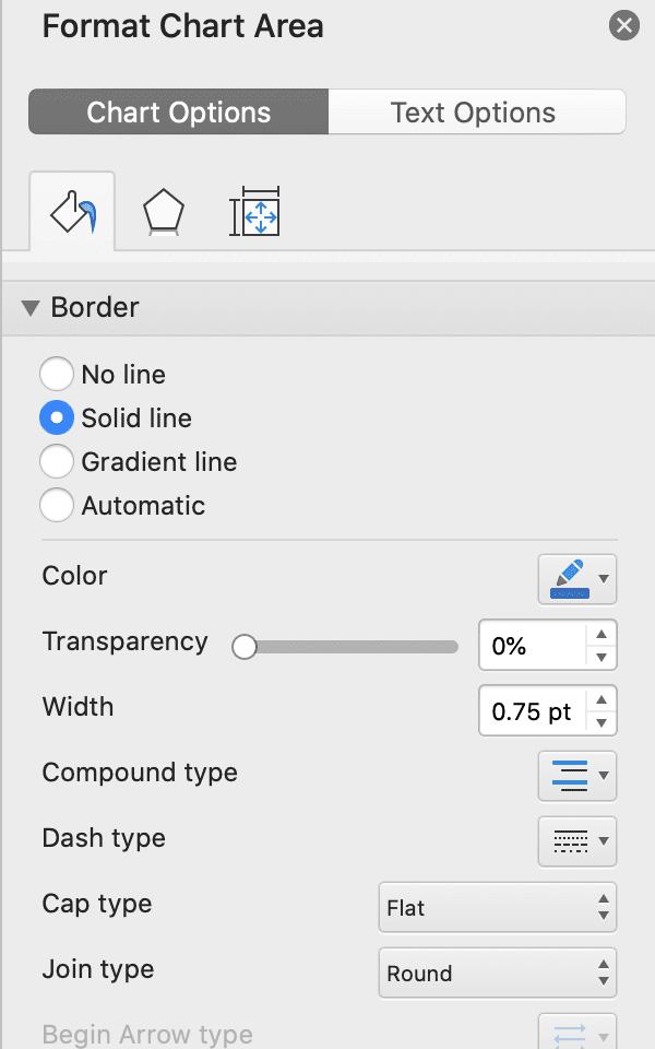
Pie Chart Border

3. Throughout the Format Chart Space, you may edit the border of your pie chart as properly — together with the border transparency, width, and shade.

Pie Chart Shadows

4. To vary the pie chart field itself (together with the field’s shadow, edges, and glow), click on on the pentagon form within the Format Chart Space sidebar.

Then, toggle the bar throughout “Transparency”, “Measurement”, “Blur”, and “Angle” till you are proud of the shadow of your pie chart field.

Pie Chart Colours

5. Click on the colour paint palette, on the prime left of excel, to vary the colours of your pie chart.

Excel provides a variety of complementary colours — together with a number of presets beneath “Colourful”, and some presets beneath “Monochromatic”. You possibly can click on between the choices till you discover a shade palette you are proud of.

(Alternatively, if you wish to change the colours of your pie chart items individually, merely double click on on the pie chart piece, toggle onto the paint part of the Format Chart Space, and select a brand new shade.)

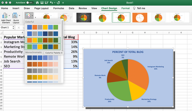
Chart Title

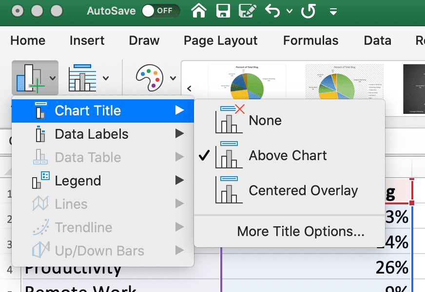
6. Change the chart title by clicking on the three bars graph icon within the prime left of excel, after which toggling to “Chart Title > None”, “Chart Title > Above Chart”, or “Chart Title > Centered Overlay”.

Change Location of Information Labels

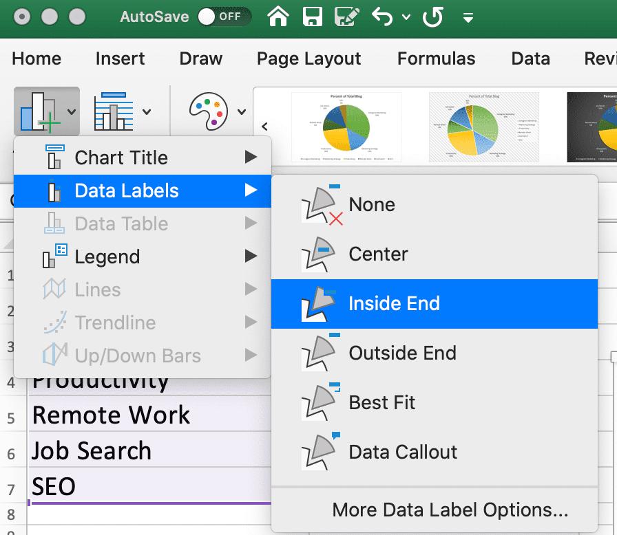
7. On the identical three bar graph icon, click on “Information Labels” to switch the place your labels seem on the pie chart. (For example, would you like the pie chart items labelled in the midst of every pie chart portion, or on the skin?)

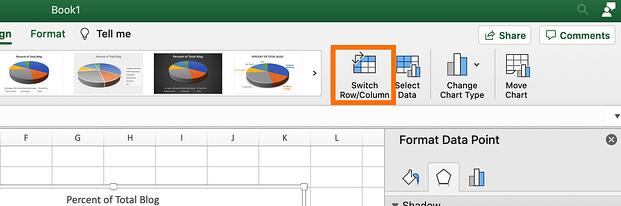
Change Row/Column

8. In the event you’d want to modify which information seems within the pie chart, click on “Change Row/Column” to see alternate data aligned out of your unique information set.

Learn how to Explode a Pie Chart in Excel

1. To blow up a chunk of your pie chart (which may also help you emphasize or draw consideration to a particular part of your pie chart), merely double-click on the piece you need to draw back.

Then, drag your cursor till it is the gap you need it, and also you’re all set!

Learn how to Create a 3D Pie Chart in Excel

1. To create a three-dimensional pie chart in excel, merely spotlight your information after which click on the “Pie” emblem.

2. Then, select the “3-D Pie” choice.

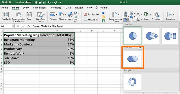
3. Lastly, select the design choice you want on the prime of your display.

Learn how to Rotate a Pie Chart in Excel

Lastly, to rotate your pie chart, double-click on the chart after which click on on the three-bar icon beneath “Format Information Level”.

Then, toggle the “Angle of first slice” till you’ve got rotated the pie chart to the diploma you need.

And there you’ve it! You are properly in your solution to creating clear, spectacular pie charts in your advertising and marketing supplies to focus on necessary information and transfer stakeholders to take motion.

In the end, you may need to experiment with all of excel’s distinctive formatting options till you determine the pie chart that works greatest in your wants. Good luck!